Tips on how to Use VLOOKUP Operate in Microsoft Excel [+ Video Tutorial]

How does VLOOKUP work?

VLOOKUP stands for “vertical lookup.” In Excel, this implies the act of trying up information vertically throughout a spreadsheet, utilizing the spreadsheet’s columns — and a singular identifier inside these columns — as the premise of your search. While you lookup your information, it should be listed vertically wherever that information is positioned.

VLOOKUP Excel Components 

VLOOKUP Excel Instance

Within the video under, we’ll present an instance in motion, utilizing the VLOOKUP operate to match e mail addresses (from a second information supply) to their corresponding information in a separate sheet. 

Creator’s observe: There are various totally different variations of Excel, so what you see within the video above won’t at all times match up precisely with what you may see in your model. That is why we encourage you to comply with together with the written directions under.

On your reference, this is what the syntax for a VLOOKUP operate seems to be like:

VLOOKUP(lookup_value , table_array , col_index_num , range_lookup)

Within the steps under, we’ll assign the correct worth to every of those parts, utilizing buyer names as our distinctive identifier to seek out the MRR of every buyer.

1. Establish a column of cells you’d wish to fill with new information.

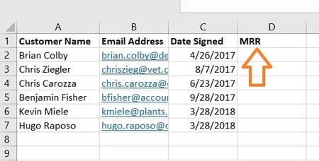
Bear in mind, you are trying to retrieve information from one other sheet and deposit it into this one. With that in thoughts, label a column subsequent to the cells you need extra data on with a correct title within the prime cell, resembling “MRR,” for month-to-month recurring income. This new column is the place the info you are fetching will go.

2. Choose ‘Operate’ (Fx) > VLOOKUP and insert this system into your highlighted cell.

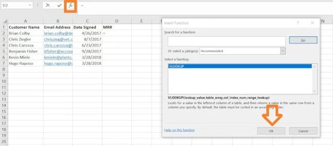
To the left of the textual content bar above your spreadsheet, you may see a small operate icon that appears like a script: Fx. Click on on the primary empty cell beneath your column title after which click on this operate icon. A field titled Components Builder or Insert Operate will seem to the correct of your display screen (relying on which model of Excel you will have).

Seek for and choose “VLOOKUP” from the listing of choices included within the Components Builder. Then, choose OK or Insert Operate to begin constructing your VLOOKUP. The cell you presently have highlighted in your spreadsheet ought to now seem like this: “=VLOOKUP()“

It’s also possible to enter this system right into a name manually by getting into the daring textual content above precisely into your required cell.

With the =VLOOKUP textual content entered into your first cell, it is time to fill the system with 4 totally different standards. These standards will assist Excel slim down precisely the place the info you need is positioned and what to search for.

3. Enter the lookup worth for which you wish to retrieve new information.

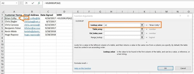
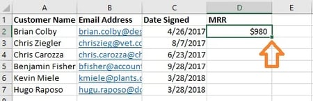
The primary standards is your lookup worth — that is the worth of your spreadsheet that has information related to it, which you need Excel to seek out and return for you. To enter it, click on on the cell that carries a worth you are looking for a match for. In our instance, proven above, it is in cell A2. You may begin migrating your new information into D2, since this cell represents the MRR of the shopper title listed in A2.

Have in mind your lookup worth might be something: textual content, numbers, web site hyperlinks, you title it. So long as the worth you are trying up matches the worth within the referring spreadsheet — which we’ll speak about that within the subsequent step — this operate will return the info you need.

4. Enter the desk array of the spreadsheet the place your required information is positioned.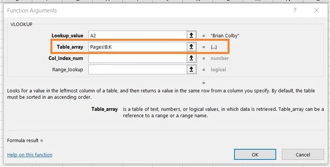

Subsequent to the “desk array” area, enter the vary of cells you want to look and the sheet the place these cells are positioned, utilizing the format proven within the screenshot above. The entry above means the info we’re on the lookout for is in a spreadsheet titled “Pages” and might be discovered wherever between column B and column Okay.

The sheet the place your information is positioned should be inside your present Excel file. This implies your information can both be in a unique desk of cells someplace in your present spreadsheet, or in a unique spreadsheet linked on the backside of your workbook, as proven under.

For instance, in case your information is positioned in “Sheet2” between cells C7 and L18, your desk array entry might be “Sheet2!C7:L18.”

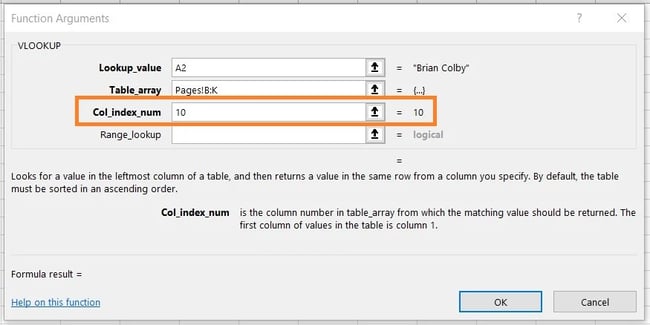
5. Enter the column variety of the info you need Excel to return.

Beneath the desk array area, you may enter the “column index quantity” of the desk array you are looking out via. For instance, in the event you’re specializing in columns B via Okay (notated “B:Okay” when entered within the “desk array” area), however the particular values you need are in column Okay, you may enter “10” within the “column index quantity” area, since column Okay is the tenth column from the left.

6. Enter your vary lookup to seek out a precise or approximate match of your lookup worth.

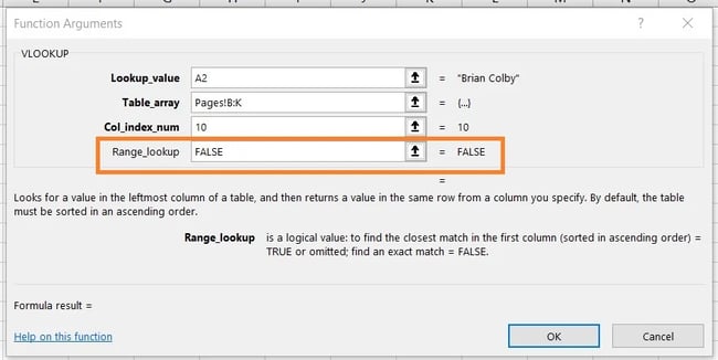
In conditions like ours, which considerations month-to-month income, you wish to discover actual matches from the desk you are looking out via. To do that, enter “FALSE” within the “vary lookup” area. This tells Excel you wish to discover solely the precise income related to every gross sales contact.

To reply your burning query: Sure, you possibly can enable Excel to search for an approximate match as a substitute of a precise match. To take action, merely enter TRUE as a substitute of FALSE within the fourth area proven above.

When VLOOKUP is ready for an approximate match, it is on the lookout for information that the majority carefully resembles your lookup worth, moderately than information that’s an identical to that worth. If you happen to’re trying up information related to a listing of web site hyperlinks, for instance, and a few of your hyperlinks have “https://” firstly, it’d behoove you to seek out an approximate match simply in case there are hyperlinks that shouldn’t have this “https://” tag. This fashion, the remainder of the hyperlink can match with out this preliminary textual content tag inflicting your VLOOKUP system to return an error if Excel cannot discover it.

7. Click on ‘Accomplished’ (or ‘Enter’) and fill your new column.

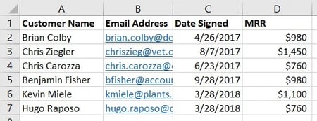
So as to formally deliver within the values you need into your new column from Step 1, click on “Accomplished” (or “Enter,” relying in your model of Excel) after filling the “vary lookup” area. It will populate your first cell. You may take this chance to look within the different spreadsheet to verify this was the right worth.

If that’s the case, populate the remainder of the brand new column with every subsequent worth by clicking the primary crammed cell, then clicking the tiny sq. that seems on the bottom-right nook of this cell. Accomplished! All of your values ought to seem.

VLOOKUP Not Working?

VLOOKUP Tutorial

Received caught after making an attempt to conduct your individual VLOOKUP with the steps above? Try this useful tutorial from Microsoft has a useful tutorial that may stroll you thru correctly utilizing the operate.