


For many entrepreneurs, attempting to arrange and analyze spreadsheets in Microsoft Excel can really feel like strolling right into a brick wall repeatedly should you’e unfamiliar with Excel formulation. You are manually replicating columns and scribbling down long-form math on a scrap of paper, all whereas considering to your self, “There has to be a greater method to do that.”
Reality be informed, there may be — you simply do not know it but.
Excel could be difficult that method. On the one hand, it is an exceptionally highly effective device for reporting and analyzing advertising information. It may well even provide help to visualize information with charts and pivot tables. On the opposite, with out the right coaching, it is easy to really feel prefer it’s working in opposition to you. For starters, there are greater than a dozen important formulation Excel can mechanically run for you so you are not combing via a whole lot of cells with a calculator in your desk.![Download 10 Excel Templates for Marketers [Free Kit]](https://no-cache.hubspot.com/cta/default/53/9ff7a4fe-5293-496c-acca-566bc6e73f42.png)
What are excel formulation?
Excel formulation provide help to establish relationships between values within the cells of your spreadsheet, carry out mathematical calculations utilizing these values, and return the ensuing worth within the cell of your alternative. Formulation you’ll be able to mechanically carry out embody sum, subtraction, share, division, common, and even dates/instances.
We’ll go over all of those, and plenty of extra, on this weblog put up.
Find out how to Insert Formulation in Excel
You may marvel what the “Formulation” tab on the highest navigation toolbar in Excel means. In newer variations of Excel, this horizontal menu — proven beneath — permits you to discover and insert Excel formulation into particular cells of your spreadsheet.
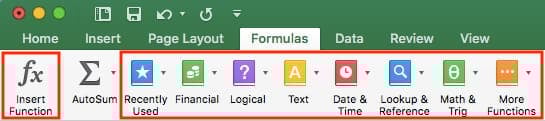
The extra you employ varied formulation in Excel, the better it’s going to be to recollect them and carry out them manually. Nonetheless, the suite of icons above is a useful catalog of formulation you’ll be able to browse and refer again to as you hone your spreadsheet abilities.
Excel formulation are additionally known as “capabilities.” To insert one into your spreadsheet, spotlight a cell by which you wish to run a method, then click on the far-left icon, “Insert Operate,” to browse standard formulation and what they do. That looking window will appear like this:
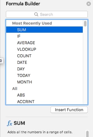 Desire a extra sorted looking expertise? Use any of the icons we have highlighted (contained in the lengthy crimson rectangle within the first screenshot above) to search out formulation associated to a wide range of widespread topics — corresponding to finance, logic, and extra. As soon as you’ve got discovered the method that fits your wants, click on “Insert Operate,” as proven within the window above.
Now, let’s do a deeper dive into among the most important Excel formulation and the way to carry out each in typical conditions.
That can assist you use Excel extra successfully (and save a ton of time), we have compiled a listing of important formulation, keyboard shortcuts, and different small methods and capabilities it’s best to know.
NOTE: The next formulation apply to the newest model of Excel. When you’re utilizing a barely older model of Excel, the placement of every characteristic talked about beneath may be barely completely different.
1. SUM
All Excel formulation start with the equals signal, =, adopted by a particular textual content tag denoting the method you need Excel to carry out.
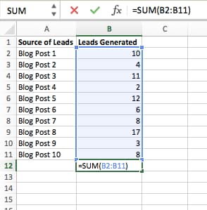
The SUM method in Excel is likely one of the most simple formulation you’ll be able to enter right into a spreadsheet, permitting you to search out the sum (or complete) of two or extra values. To carry out the SUM method, enter the values you need so as to add collectively utilizing the format, =SUM(worth 1, worth 2, and so forth).
The values you enter into the SUM method can both be precise numbers or equal to the quantity in a particular cell of your spreadsheet.
- To search out the SUM of 30 and 80, for instance, sort the next method right into a cell of your spreadsheet: =SUM(30, 80). Press “Enter,” and the cell will produce the full of each numbers: 110.
- To search out the SUM of the values in cells B2 and B11, for instance, sort the next method right into a cell of your spreadsheet: =SUM(B2, B11). Press “Enter,” and the cell will produce the full of the numbers at present stuffed in cells B2 and B11. If there aren’t any numbers in both cell, the method will return 0.
Have in mind you may as well discover the full worth of a checklist of numbers in Excel. To search out the SUM of the values in cells B2 via B11, sort the next method right into a cell of your spreadsheet: =SUM(B2:B11). Word the colon between each cells, moderately than a comma. See how this may look in an Excel spreadsheet for a content material marketer, beneath:
2. IF
The IF method in Excel is denoted =IF(logical_test, value_if_true, value_if_false). This lets you enter a textual content worth into the cell “if” one thing else in your spreadsheet is true or false. For instance, =IF(D2=”Gryffindor”,”10″,”0″) would award 10 factors to cell D2 if that cell contained the phrase “Gryffindor.”
There are occasions after we wish to know what number of instances a worth seems in our spreadsheets. However there are additionally these instances after we wish to discover the cells that comprise these values, and enter particular information subsequent to it.
We’ll return to Sprung’s instance for this one. If we wish to award 10 factors to everybody who belongs within the Gryffindor home, as an alternative of manually typing in 10’s subsequent to every Gryffindor pupil’s identify, we’ll use the IF-THEN method to say: If the coed is in Gryffindor, then she or he ought to get ten factors.
- The method: IF(logical_test, value_if_true, value_if_false)
- Logical_Test: The logical take a look at is the “IF” a part of the assertion. On this case, the logic is D2=”Gryffindor.” Ensure that your Logical_Test worth is in citation marks.
- Value_if_True: If the worth is true — that’s, if the coed lives in Gryffindor — this worth is the one which we wish to be displayed. On this case, we wish it to be the quantity 10, to point that the coed was awarded the ten factors. Word: Solely use citation marks if you’d like the consequence to be textual content as an alternative of a quantity.
- Value_if_False: If the worth is fake — and the coed does not reside in Gryffindor — we wish the cell to point out “0,” for 0 factors.
- Formulation in beneath instance: =IF(D2=”Gryffindor”,”10″,”0″)
3. Proportion
To carry out the proportion method in Excel, enter the cells you are discovering a share for within the format, =A1/B1. To transform the ensuing decimal worth to a share, spotlight the cell, click on the House tab, and choose “Proportion” from the numbers dropdown.
There is not an Excel “method” for percentages per se, however Excel makes it straightforward to transform the worth of any cell right into a share so you are not caught calculating and reentering the numbers your self.
The fundamental setting to transform a cell’s worth right into a share is underneath Excel’s House tab. Choose this tab, spotlight the cell(s) you’d wish to convert to a share, and click on into the dropdown menu subsequent to Conditional Formatting (this menu button may say “Common” at first). Then, choose “Proportion” from the checklist of choices that seems. This can convert the worth of every cell you’ve got highlighted right into a share. See this characteristic beneath.
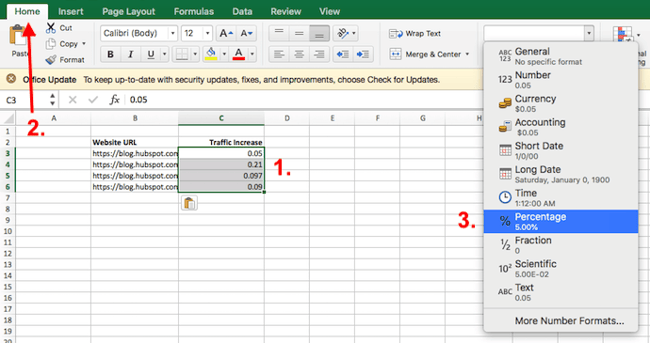
Have in mind should you’re utilizing different formulation, such because the division method (denoted =A1/B1), to return new values, your values may present up as decimals by default. Merely spotlight your cells earlier than or after you carry out this method, and set these cells’ format to “Proportion” from the House tab — as proven above.
4. Subtraction
To carry out the subtraction method in Excel, enter the cells you are subtracting within the format, =SUM(A1, -B1). This can subtract a cell utilizing the SUM method by including a unfavorable signal earlier than the cell you are subtracting. For instance, if A1 was 10 and B1 was 6, =SUM(A1, -B1) would carry out 10 + -6, returning a worth of 4.
Like percentages, subtracting would not have its personal method in Excel both, however that does not imply it could actually’t be achieved. You’ll be able to subtract any values (or these values inside cells) two other ways.
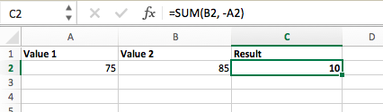
- Utilizing the =SUM method. To subtract a number of values from each other, enter the cells you’d wish to subtract within the format =SUM(A1, -B1), with a unfavorable signal (denoted with a hyphen) earlier than the cell whose worth you are subtracting. Press enter to return the distinction between each cells included within the parentheses. See how this appears within the screenshot above.
- Utilizing the format, =A1-B1. To subtract a number of values from each other, merely sort an equals signal adopted by your first worth or cell, a hyphen, and the worth or cell you are subtracting. Press Enter to return the distinction between each values.
5. Multiplication
To carry out the multiplication method in Excel, enter the cells you are multiplying within the format, =A1*B1. This method makes use of an asterisk to multiply cell A1 by cell B1. For instance, if A1 was 10 and B1 was 6, =A1*B1 would return a worth of 60.
You may suppose multiplying values in Excel has its personal method or makes use of the “x” character to indicate multiplication between a number of values. Really, it is as straightforward as an asterisk — *.
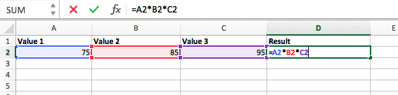
To multiply two or extra values in an Excel spreadsheet, spotlight an empty cell. Then, enter the values or cells you wish to multiply collectively within the format, =A1*B1*C1 … and so forth. The asterisk will successfully multiply every worth included within the method.
Press Enter to return your required product. See how this appears within the screenshot above.
6. Division
To carry out the division method in Excel, enter the cells you are dividing within the format, =A1/B1. This method makes use of a ahead slash, “/,” to divide cell A1 by cell B1. For instance, if A1 was 5 and B1 was 10, =A1/B1 would return a decimal worth of 0.5.
Division in Excel is likely one of the easiest capabilities you’ll be able to carry out. To take action, spotlight an empty cell, enter an equals signal, “=,” and comply with it up with the 2 (or extra) values you’d wish to divide with a ahead slash, “/,” in between. The consequence must be within the following format: =B2/A2, as proven within the screenshot beneath.
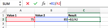
Hit Enter, and your required quotient ought to seem within the cell you initially highlighted.
7. DATE
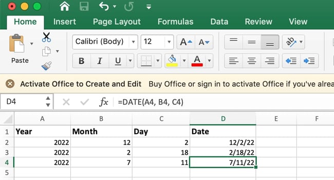
The Excel DATE method is denoted =DATE(12 months, month, day). This method will return a date that corresponds to the values entered within the parentheses — even values referred from different cells. For instance, if A1 was 2018, B1 was 7, and C1 was 11, =DATE(A1,B1,C1) would return 7/11/2018.
Creating dates within the cells of an Excel spreadsheet generally is a fickle process once in a while. Fortunately, there is a useful method to make formatting your dates straightforward. There are two methods to make use of this method:
- Create dates from a collection of cell values. To do that, spotlight an empty cell, enter “=DATE,” and in parentheses, enter the cells whose values create your required date — beginning with the 12 months, then the month quantity, then the day. The ultimate format ought to appear like this: =DATE(12 months, month, day). See how this appears within the screenshot beneath.
- Mechanically set at this time’s date. To do that, spotlight an empty cell and enter the next string of textual content: =DATE(YEAR(TODAY()), MONTH(TODAY()), DAY(TODAY())). Urgent enter will return the present date you are working in your Excel spreadsheet.
In both utilization of Excel’s date method, your returned date must be within the type of “mm/dd/yy” — until your Excel program is formatted in a different way.
8. Array
An array method in Excel surrounds a easy method in brace characters utilizing the format, {=(Begin Worth 1:Finish Worth 1)*(Begin Worth 2:Finish Worth 2)}. By urgent ctrl+shift+heart, this may calculate and return worth from a number of ranges, moderately than simply particular person cells added to or multiplied by each other.
Calculating the sum, product, or quotient of particular person cells is straightforward — simply use the =SUM method and enter the cells, values, or vary of cells you wish to carry out that arithmetic on. However what about a number of ranges? How do you discover the mixed worth of a giant group of cells?
Numerical arrays are a helpful approach to carry out a couple of method on the identical time in a single cell so you’ll be able to see one last sum, distinction, product, or quotient. When you’re seeking to discover complete gross sales income from a number of offered models, for instance, the array method in Excel is ideal for you. Here is the way you’d do it:
- To begin utilizing the array method, sort “=SUM,” and in parentheses, enter the first of two (or three, or 4) ranges of cells you’d wish to multiply collectively. Here is what your progress may appear like: =SUM(C2:C5
- Subsequent, add an asterisk after the final cell of the primary vary you included in your method. This stands for multiplication. Following this asterisk, enter your second vary of cells. You may be multiplying this second vary of cells by the primary. Your progress on this method ought to now appear like this: =SUM(C2:C5*D2:D5)
- Able to press Enter? Not so quick … As a result of this method is so sophisticated, Excel reserves a special keyboard command for arrays. As soon as you’ve got closed the parentheses in your array method, press Ctrl+Shift+Enter. This can acknowledge your method as an array, wrapping your method in brace characters and efficiently returning your product of each ranges mixed.
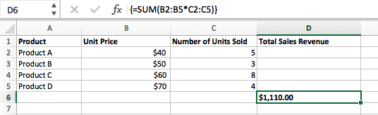
In income calculations, this will minimize down in your effort and time considerably. See the ultimate method within the screenshot above.
9. COUNT
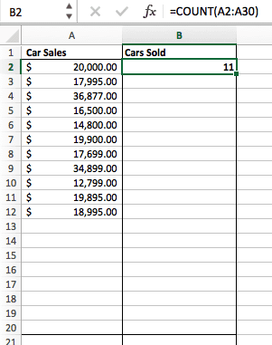
The COUNT method in Excel is denoted =COUNT(Begin Cell:Finish Cell). This method will return a worth that is the same as the variety of entries discovered inside your required vary of cells. For instance, if there are eight cells with entered values between A1 and A10, =COUNT(A1:A10) will return a worth of 8.
The COUNT method in Excel is especially helpful for giant spreadsheets, whereby you wish to see what number of cells comprise precise entries. Do not be fooled: This method will not do any math on the values of the cells themselves. This method is solely to learn the way many cells in a specific vary are occupied with one thing.
Utilizing the method in daring above, you’ll be able to simply run a rely of energetic cells in your spreadsheet. The consequence will look slightly one thing like this:
10. AVERAGE
To carry out the typical method in Excel, enter the values, cells, or vary of cells of which you are calculating the typical within the format, =AVERAGE(number1, number2, and so forth.) or =AVERAGE(Begin Worth:Finish Worth). This can calculate the typical of all of the values or vary of cells included within the parentheses.
Discovering the typical of a variety of cells in Excel retains you from having to search out particular person sums after which performing a separate division equation in your complete. Utilizing =AVERAGE as your preliminary textual content entry, you’ll be able to let Excel do all of the give you the results you want.
For reference, the typical of a bunch of numbers is the same as the sum of these numbers, divided by the variety of objects in that group.
11. SUMIF
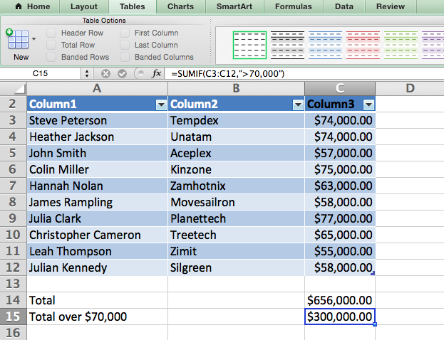
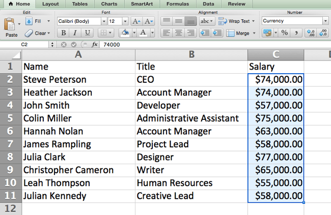
The SUMIF method in Excel is denoted =SUMIF(vary, standards, [sum range]). This can return the sum of the values inside a desired vary of cells that every one meet one criterion. For instance, =SUMIF(C3:C12,”>70,000″) would return the sum of values between cells C3 and C12 from solely the cells which are higher than 70,000.
For example you wish to decide the revenue you generated from a listing of leads who’re related to particular space codes, or calculate the sum of sure staff’ salaries — however provided that they fall above a specific quantity. Doing that manually sounds a bit time-consuming, to say the least.
With the SUMIF operate, it would not should be — you’ll be able to simply add up the sum of cells that meet sure standards, like within the wage instance above.
- The method: =SUMIF(vary, standards, [sum_range])
- Vary: The vary that’s being examined utilizing your standards.
- Standards: The factors that decide which cells in Criteria_range1 will probably be added collectively
- [Sum_range]: An elective vary of cells you are going to add up along with the primary Vary entered. This subject could also be omitted.
Within the instance beneath, we needed to calculate the sum of the salaries that had been higher than $70,000. The SUMIF operate added up the greenback quantities that exceeded that quantity within the cells C3 via C12, with the method =SUMIF(C3:C12,”>70,000″).
12. TRIM
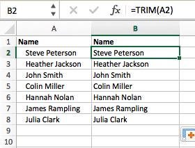
The TRIM method in Excel is denoted =TRIM(textual content). This method will take away any areas entered earlier than and after the textual content entered within the cell. For instance, if A2 contains the identify ” Steve Peterson” with undesirable areas earlier than the primary identify, =TRIM(A2) would return “Steve Peterson” with no areas in a brand new cell.
Electronic mail and file sharing are fantastic instruments in at this time’s office. That’s, till one in all your colleagues sends you a worksheet with some actually funky spacing. Not solely can these rogue areas make it troublesome to seek for information, however additionally they have an effect on the outcomes if you attempt to add up columns of numbers.
Slightly than painstakingly eradicating and including areas as wanted, you’ll be able to clear up any irregular spacing utilizing the TRIM operate, which is used to take away further areas from information (apart from single areas between phrases).
- The method: =TRIM(textual content).
- Textual content: The textual content or cell from which you wish to take away areas.
Here is an instance of how we used the TRIM operate to take away further areas earlier than a listing of names. To take action, we entered =TRIM(“A2”) into the Formulation Bar, and replicated this for every identify beneath it in a brand new column subsequent to the column with undesirable areas.
Under are another Excel formulation you may discover helpful as your information administration wants develop.
13. LEFT, MID, and RIGHT
For example you’ve gotten a line of textual content inside a cell that you just wish to break down into a couple of completely different segments. Slightly than manually retyping every bit of the code into its respective column, customers can leverage a collection of string capabilities to deconstruct the sequence as wanted: LEFT, MID, or RIGHT.
LEFT
- Function: Used to extract the primary X numbers or characters in a cell.
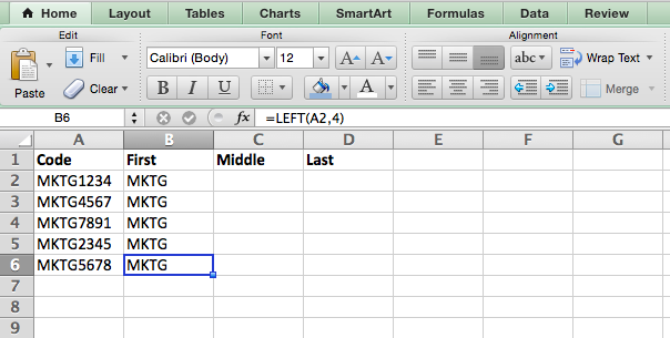
- The method: =LEFT(textual content, number_of_characters)
- Textual content: The string that you just want to extract from.
- Number_of_characters: The variety of characters that you just want to extract ranging from the left-most character.
Within the instance beneath, we entered =LEFT(A2,4) into cell B2, and copied it into B3:B6. That allowed us to extract the primary 4 characters of the code.
MID
- Function: Used to extract characters or numbers within the center based mostly on place.
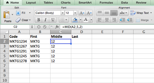
- The method: =MID(textual content, start_position, number_of_characters)
- Textual content: The string that you just want to extract from.
- Start_position: The place within the string that you just wish to start extracting from. For instance, the primary place within the string is 1.
- Number_of_characters: The variety of characters that you just want to extract.
On this instance, we entered =MID(A2,5,2) into cell B2, and copied it into B3:B6. That allowed us to extract the 2 numbers beginning within the fifth place of the code.
RIGHT
- Function: Used to extract the final X numbers or characters in a cell.
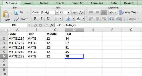
- The method: =RIGHT(textual content, number_of_characters)
- Textual content: The string that you just want to extract from.
- Number_of_characters: The variety of characters that you just wish to extract ranging from the right-most character.
For the sake of this instance, we entered =RIGHT(A2,2) into cell B2, and copied it into B3:B6. That allowed us to extract the final two numbers of the code.
14. VLOOKUP
This one is an oldie, however a goodie — and it’s kind of extra in depth than among the different formulation we have listed right here. However it’s particularly useful for these instances when you’ve gotten two units of information on two completely different spreadsheets, and wish to mix them right into a single spreadsheet.
My colleague, Rachel Sprung — whose “Find out how to Use Excel” tutorial is a must-read for anybody who needs to be taught — makes use of a listing of names, e mail addresses, and firms for instance. If in case you have a listing of individuals’s names subsequent to their e mail addresses in a single spreadsheet, and a listing of those self same folks’s e mail addresses subsequent to their firm names within the different, however you need the names, e mail addresses, and firm names of these folks to seem in a single place — that is the place VLOOKUP is available in.
Word: When utilizing this method, you have to be sure that no less than one column seems identically in each spreadsheets. Scour your information units to verify the column of information you are utilizing to mix your data is strictly the identical, together with no further areas.
- The method: VLOOKUP(lookup worth, desk array, column quantity, [range lookup])
- Lookup Worth: The equivalent worth you’ve gotten in each spreadsheets. Select the primary worth in your first spreadsheet. In Sprung’s instance that follows, this implies the primary e mail deal with on the checklist, or cell 2 (C2).
- Desk Array: The vary of columns on Sheet 2 you are going to pull your information from, together with the column of information equivalent to your lookup worth (in our instance, e mail addresses) in Sheet 1 in addition to the column of information you are attempting to repeat to Sheet 1. In our instance, that is “Sheet2!A:B.” “A” means Column A in Sheet 2, which is the column in Sheet 2 the place the info equivalent to our lookup worth (e mail) in Sheet 1 is listed. The “B” means Column B, which incorporates the data that is solely out there in Sheet 2 that you just wish to translate to Sheet 1.
- Column Quantity: The desk array tells Excel the place (which column) the brand new information you wish to copy to Sheet 1 is positioned. In our instance, this is able to be the “Home” column, the second in our desk array, making it column quantity 2.
- Vary Lookup: Use FALSE to make sure you pull in solely precise worth matches.
- The method with variables from Sprung’s instance beneath: =VLOOKUP(C2,Sheet2!A:B,2,FALSE)
On this instance, Sheet 1 and Sheet 2 comprise lists describing completely different details about the identical folks, and the widespread thread between the 2 is their e mail addresses. For example we wish to mix each datasets so that every one the home data from Sheet 2 interprets over to Sheet 1. Here is how that might work:
15. RANDOMIZE
There is a nice article that likens Excel’s RANDOMIZE method to shuffling a deck of playing cards. All the deck is a column, and every card — 52 in a deck — is a row. “To shuffle the deck,” writes Steve McDonnell, “you’ll be able to compute a brand new column of information, populate every cell within the column with a random quantity, and kind the workbook based mostly on the random quantity subject.”
In advertising, you may use this characteristic if you wish to assign a random quantity to a listing of contacts — like should you needed to experiment with a brand new e mail marketing campaign and had to make use of blind standards to pick out who would obtain it. By assigning numbers to stated contacts, you would apply the rule, “Any contact with a determine of 6 or above will probably be added to the brand new marketing campaign.”
- The method: RAND()
- Begin with a single column of contacts. Then, within the column adjoining to it, sort “RAND()” — with out the citation marks — beginning with the highest contact’s row.
-
- RANDBETWEEN permits you to dictate the vary of numbers that you just wish to be assigned. Within the case of this instance, I needed to make use of one via 10.
- backside: The bottom quantity within the vary.
- high: The best quantity within the vary,For the instance beneath: RANDBETWEEN(backside,high)
- Formulation in beneath instance: =RANDBETWEEN(1,10)
Useful stuff, proper? Now for the icing on the cake: As soon as you’ve got mastered the Excel method you want, you may wish to replicate it for different cells with out rewriting the method. And fortunately, there’s an Excel operate for that, too. Test it out beneath.
Generally, you may wish to run the identical method throughout a whole row or column of your spreadsheet. For example, for instance, you have a listing of numbers in columns A and B of a spreadsheet and wish to enter particular person totals of every row into column C.
Clearly, it will be too tedious to regulate the values of the method for every cell so that you’re discovering the full of every row’s respective numbers. Fortunately, Excel permits you to mechanically full the column; all you need to do is enter the method within the first row. Take a look at the next steps:
- Sort your method into an empty cell and press “Enter” to run the method.
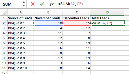
- Hover your cursor over the bottom-right nook of the cell containing the method. You may see a small, daring “+” image seem.
- Whilst you can double-click this image to mechanically fill the whole column together with your method, you may as well click on and drag your cursor down manually to fill solely a particular size of the column.
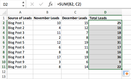 As soon as you’ve got reached the final cell within the column you’d wish to enter your method, launch your mouse to repeat the method. Then, merely test every new worth to make sure it corresponds to the proper cells.
Excel Keyboard Shortcuts
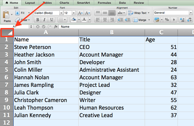
1. Shortly choose rows, columns, or the entire spreadsheet.
Maybe you are crunched for time. I imply, who is not? No time, no drawback. You’ll be able to choose your total spreadsheet in only one click on. All you need to do is solely click on the tab within the top-left nook of your sheet to spotlight every little thing all of sudden.
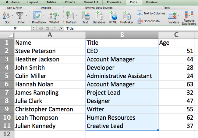
Simply wish to choose every little thing in a specific column or row? That is simply as straightforward with these shortcuts:
For Mac:
- Choose Column = Command + Shift + Down/Up
- Choose Row = Command + Shift + Proper/Left
For PC:
- Choose Column = Management + Shift + Down/Up
- Choose Row = Management + Shift + Proper/Left
This shortcut is very useful if you’re working with bigger information units, however solely want to pick out a particular piece of it.
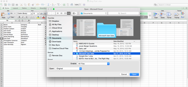
2. Shortly open, shut, or create a workbook.
Must open, shut, or create a workbook on the fly? The next keyboard shortcuts will allow you to finish any of the above actions in lower than a minute’s time.
For Mac:
- Open = Command + O
- Shut = Command + W
- Create New = Command + N
For PC:
- Open = Management + O
- Shut = Management + F4
- Create New = Management + N
3. Format numbers into forex.
Have uncooked information that you just wish to flip into forex? Whether or not it’s wage figures, advertising budgets, or ticket gross sales for an occasion, the answer is straightforward. Simply spotlight the cells you want to reformat, and choose Management + Shift + $.
The numbers will mechanically translate into greenback quantities — full with greenback indicators, commas, and decimal factors.
Word: This shortcut additionally works with percentages. If you wish to label a column of numerical values as “p.c” figures, substitute “$” with “%”.
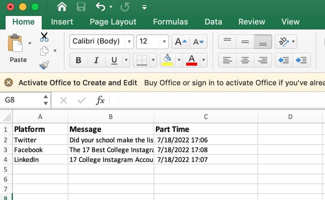
4. Insert present date and time right into a cell.
Whether or not you are logging social media posts, or protecting observe of duties you are checking off your to-do checklist, you may wish to add a date and time stamp to your worksheet. Begin by choosing the cell to which you wish to add this data.
Then, relying on what you wish to insert, do one of many following:
- Insert present date = Management + ; (semi-colon)
- Insert present time = Management + Shift + ; (semi-colon)
- Insert present date and time = Management + ; (semi-colon), SPACE, after which Management + Shift + ; (semi-colon).
Different Excel Tips
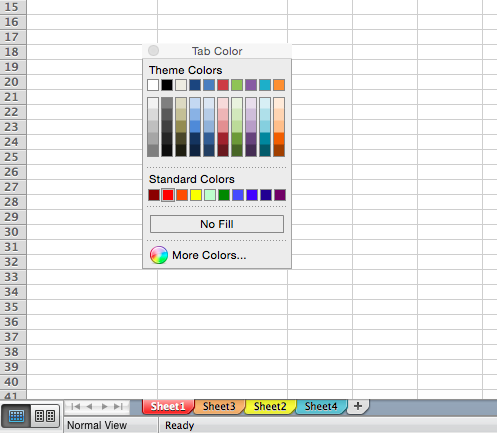
1. Customise the colour of your tabs.
When you’ve acquired a ton of various sheets in a single workbook — which occurs to the most effective of us — make it simpler to establish the place you might want to go by color-coding the tabs. For instance, you may label final month’s advertising stories with crimson, and this month’s with orange.
Merely proper click on a tab and choose “Tab Shade.” A popup will seem that permits you to select a shade from an present theme, or customise one to satisfy your wants.
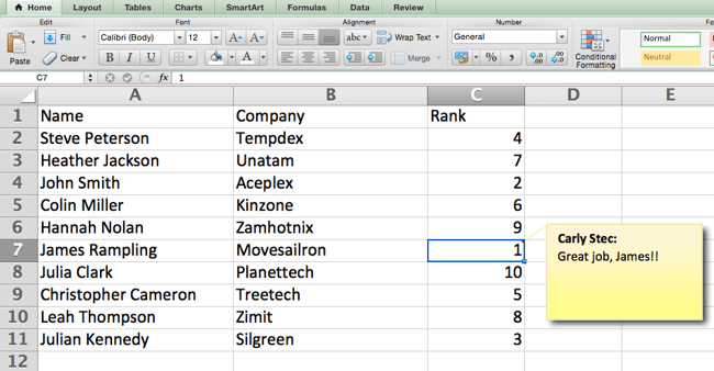
2. Add a remark to a cell.
Whenever you wish to make an observation or add a remark to a particular cell inside a worksheet, merely right-click the cell you wish to touch upon, then click on Insert Remark. Sort your remark into the textual content field, and click on outdoors the remark field to reserve it.
Cells that comprise feedback show a small, crimson triangle within the nook. To view the remark, hover over it.
3. Copy and duplicate formatting.
When you’ve ever spent a while formatting a sheet to your liking, you in all probability agree that it is not precisely essentially the most pleasing exercise. In actual fact, it is fairly tedious.
For that purpose, it is seemingly that you do not wish to repeat the method subsequent time — nor do you need to. Because of Excel’s Format Painter, you’ll be able to simply copy the formatting from one space of a worksheet to a different.
Choose what you need to duplicate, then choose the Format Painter possibility — the paintbrush icon — from the dashboard. The pointer will then show a paintbrush, prompting you to pick out the cell, textual content, or total worksheet to which you wish to apply that formatting, as proven beneath:
.gif?width=650&name=Copy%20Duplicate%20Formatting%20(1).gif)
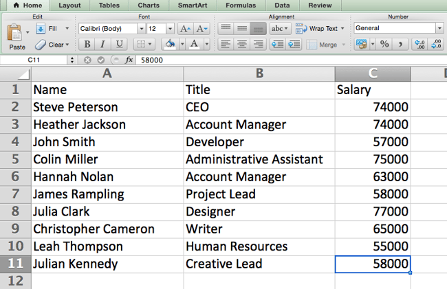
4. Determine duplicate values.
In lots of cases, duplicate values — like duplicate content material when managing search engine optimization — could be troublesome if gone uncorrected. In some instances, although, you merely want to pay attention to it.
Regardless of the scenario could also be, it is easy to floor any present duplicate values inside your worksheet in just some fast steps. To take action, click on into the Conditional Formatting possibility, and choose Spotlight Cell Guidelines > Duplicate Values
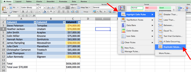
Utilizing the popup, create the specified formatting rule to specify which kind of duplicate content material you want to convey ahead.
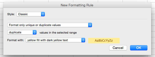
Within the instance above, we had been seeking to establish any duplicate salaries throughout the chosen vary, and formatted the duplicate cells in yellow.
Excel Shortcuts Save You Time
In advertising, using Excel is fairly inevitable — however with these methods, it would not should be so daunting. As they are saying, observe makes good. The extra you employ these formulation, shortcuts, and methods, the extra they’re going to turn into second nature.
Editor’s be aware: This put up was initially revealed in January 2019 and has been up to date for comprehensiveness.


